In the first part of this series, I talked about what sound is and how a sound can be represented in analogue equipment. In this part of the series I’ll discuss how a sound can be represented digitally.
First though, it is necessary to cover some of the fundamental theory of waveforms so that you have a full understanding of the terminology being used.
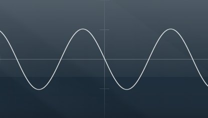
Here is a simple waveform.
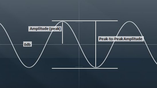
The strength of an audio signal is normally measured in decibels relative to a 0db level at which no sound is heard. The 0db reference level is usually represented by a line running horizontally through the waveform. The further the waveform moves above or below this line, the louder the signal is. The distance between the 0db level and the peak of a waveform is known as the peak amplitude of the waveform. The distance between the peak of a waveform and the corresponding trough is the peak-to-peak amplitude.
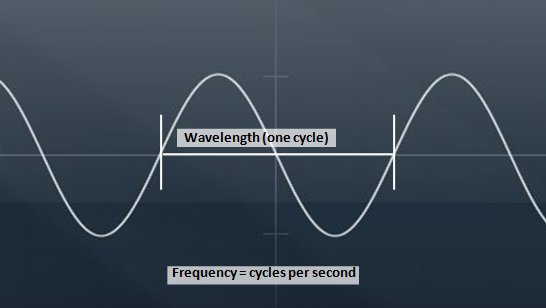
The period in which the waveform passes from the 0db level to its peak, through the 0db level to its trough and back to the 0db level again is a single cycle of the waveform. The number of times the waveform cycles every second is the waveform’s frequency. Finally, the distance between the same point on two consecutive cycles of the waveform is known as the wavelength. The wavelength is inversely proportional to the frequency. So as the wavelength decreases the frequency increases.
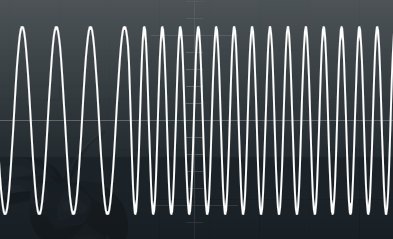
The oscilloscope trace below shows the wavelength getting shorter as the frequency increases.
Having established those basic principles, it is now possible to look at how the representation of sound in analogue and digital systems differs.
To begin with it is important to understand the difference between analogue and digital systems. An analogue system has a continuously variable state. For example, in an electrical circuit the state of the circuit might vary continuously between -10 and +10 volts. A digital system’s state is defined as a series of discrete numbers. For example, a pocket calculator’s memory might be able to store 1024 numbers between 0 and 65535.
You will recall that when a waveform was represented in an analogue system, the shape of the wave could be reproduced very closely by having the circuit’s voltage change to match the changes in the waveform. If you want to represent a waveform in a digital system then it has to be represented as a series of discrete numbers. This is achieved by a device known as an analogue-to-digital convertor (often abbreviated to ADC or A/D).
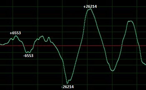
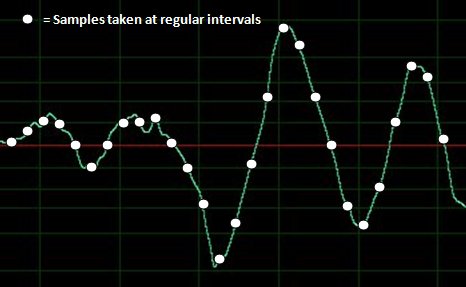
This works by sampling the waveform at regular intervals it and representing the level of the waveform at each point with a number. Let’s say, for the sake of argument, that a particular digital system has a numerical range of -32767 to 32768. When the waveform has a small non-zero amplitude, this might be represented by +6553 or -6553, while a larger non-zero amplitude might be represented by +26214 or -26214, as the following diagram shows.
The process of taking an analogue waveform and converting it into a series of numbers is called sampling. The frequency with which the ADC works is known as the sampling rate. For example, music intended to be reproduced on a compact disc is sampled at 44.1 Khz (i.e. the ADC samples the waveform 44,100 times every second).
To reproduce a sound, once it has been stored digitally, the series of numbers representing the waveform must be converted back to a continuously variable (analogue) form, for example a variable voltage that can be used to drive the cone in a speaker. This is achieved with another device known as a digital-to-analogue converter (often abbreviated to DAC or D/A).
The DAC takes each number and uses it to set the state of the circuit to an appropriate level. For example, +6553 might be converted to +2 volts, while -26214 might be converted to -8 volts. As you might expect, for the results to be meaningful the DAC should convert the samples back at the same frequency (or sampling rate) that the ADC has used.
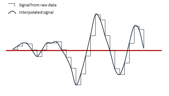
A point to note here is that the DAC cannot simply hold the voltage of the circuit at the relevant level until it reads the next sample. If it did so there would be sudden jumps in the voltage between one sample and the next and this would be heard as distortion when the sound was reproduced by the speaker.
To overcome this, the DAC uses a process known as interpolation. This is the process whereby the DAC applies a mathematical algorithm to create a smooth curve between data points. This will result in the voltage in the circuit transitioning smoothly and continuously between one data point and the next, which results in a distortion free reproduction of the original sound.
The quality of the interpolation algorithm will affect the quality of reproduction. However, the quality of reproduction is also affected by two other factors:
- the sampling rate (how frequently the waveform is sampled)
- the resolution (how many discrete values can be used to represent the shape of the waveform).
Consider these in turn.
Sampling Rate
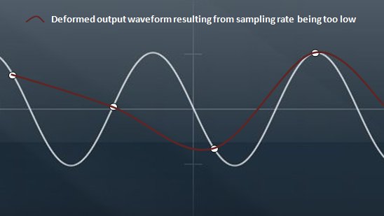
Generally speaking the faster you are able to sample a waveform, the better the quality of the reproduction will be. As the sampling rate is lowered, less of the detail of the original waveform is able to be captured, so when the data is converted back, the resulting waveform will be cruder than the original waveform. What happens is that the higher frequency components of the signal become degraded, which makes the sound less bright. Furthermore, when the signal is converted back, additional high frequencies, not present in the original waveform, are introduced, thus adding unwanted noise to the signal. This is known as aliasing.
First listen to this original sound sample at 44.1Khz.
Now listen to the sound again with increasingly lower sample rates. You will be able to hear the quality of the signal degrade as more noise is introduced and the original high frequency sounds become attenuated.
22050Hz
11025Hz
8000Hz
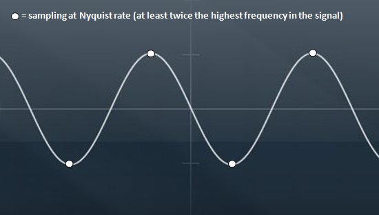
The engineer Harry Nyquist came up with a theorem for avoiding aliasing. In a nutshell the theorem requires that the sampling frequency is at least twice that of the highest frequency in the waveform to be sampled. This is known as the Nyquist Rate. You can see that this results in at least two data points being taken for each cycle in the waveform, which is sufficient to reproduce all the frequencies accurately when the waveform is recreated.
If you consider that the range of human hearing is approximately 20Hz to 20Khz you can understand why the sampling rate selected for compact disc technology was 44.1Khz. This rate allows all the frequencies normally heard by humans to be accurately reproduced.
Resolution
Resolution refers to the number of discrete values that can be used to represent the waveform’s amplitude range. As most digital systems are binary, this is usually measured in binary digits or bits. The resolution of a compact disc, for example, is 16 bits. This allows for 65536 discrete values to represent the entire amplitude range of the signal. Generally speaking, the greater the resolution the more faithfully the dynamic range of the original waveform can be reproduced. As the resolution is decreased, the reproduction of the waveform will lose much of the dynamic subtlety of the original.
Listen again to the original recording.
Now listen to the same recording with a resolution of 8-bits.
The difference is more subtle in this case, but through a good quality audio system and speakers you can hear that the dynamic reproduction is poorer.
In the next part of this series I’ll discuss audio waveforms in more detail and show how complex waveforms can be created from simple waveforms using a process known as additive synthesis.
The images in this series were created by me using a variety of graphics tools. The audio clips in this article were assembled by me from stock clips using a variety of audio tools.
Be First to Comment